05 - First order acoustic modeling on a staggered grid
from devito import *
from examples.seismic.source import DGaussSource, TimeAxis
from examples.seismic import plot_image
import numpy as np

from sympy import init_printing
init_printing(use_latex='mathjax')
# Initial grid: 1km x 1km, with spacing 100m
extent = (2000., 2000.)
shape = (81, 81)
x = SpaceDimension(name='x', spacing=Constant(name='h_x', value=extent[0]/(shape[0]-1)))
z = SpaceDimension(name='z', spacing=Constant(name='h_z', value=extent[1]/(shape[1]-1)))
grid = Grid(extent=extent, shape=shape, dimensions=(x, z))
# Timestep size from Eq. 7 with V_p=6000. and dx=100
t0, tn = 0., 200.
dt = 1e2*(1. / np.sqrt(2.)) / 60.
time_range = TimeAxis(start=t0, stop=tn, step=dt)
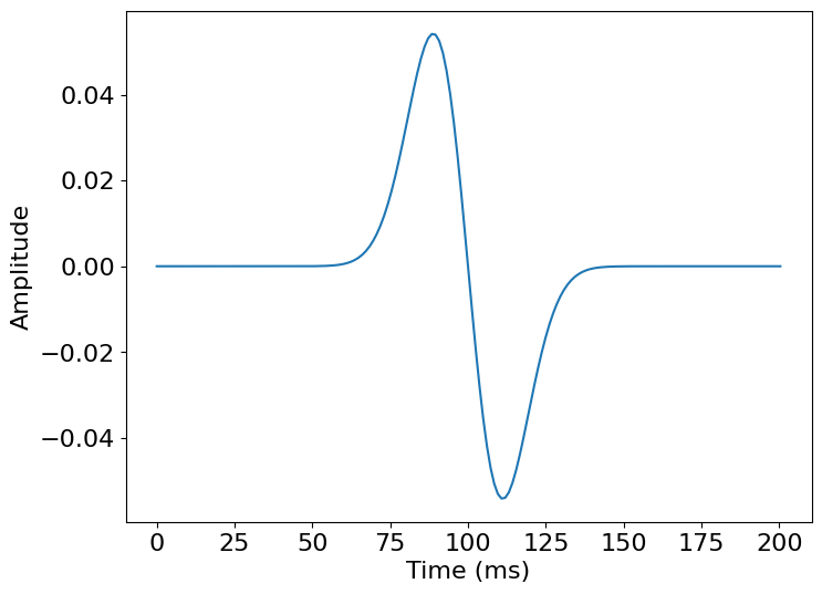
src = DGaussSource(name='src', grid=grid, f0=0.01, time_range=time_range, a=0.004)
src.coordinates.data[:] = [1000., 1000.]
# NBVAL_SKIP

src.show()
# Now we create the velocity and pressure fields
p = TimeFunction(name='p', grid=grid, staggered=NODE, space_order=2, time_order=1)
v = VectorTimeFunction(name='v', grid=grid, space_order=2, time_order=1)
from devito.finite_differences.operators import div, grad
t = grid.stepping_dim
time = grid.time_dim

# We need some initial conditions
V_p = 4.0
density = 1.

ro = 1/density
l2m = V_p*V_p*density

# The source injection term
src_p = src.inject(field=p.forward, expr=src)

# 2nd order acoustic according to fdelmoc
u_v_2 = Eq(v.forward, solve(v.dt - ro * grad(p), v.forward))
u_p_2 = Eq(p.forward, solve(p.dt - l2m * div(v.forward), p.forward))
u_v_2
\displaystyle \left[\begin{matrix}v_x(t + dt, x + h_x/2, z)\\v_z(t + dt, x, z + h_z/2)\end{matrix}\right] = \left[\begin{matrix}dt \left(\frac{\partial}{\partial x} p(t, x, z) + \frac{v_x(t, x + h_x/2, z)}{dt}\right)\\dt \left(\frac{\partial}{\partial z} p(t, x, z) + \frac{v_z(t, x, z + h_z/2)}{dt}\right)\end{matrix}\right]
u_p_2
\displaystyle p(t + dt, x, z) = dt \left(16.0 \frac{\partial}{\partial x} v_x(t + dt, x + h_x/2, z) + 16.0 \frac{\partial}{\partial z} v_z(t + dt, x, z + h_z/2) + \frac{p(t, x, z)}{dt}\right)
op_2 = Operator([u_v_2, u_p_2] + src_p)
# NBVAL_IGNORE_OUTPUT

# Propagate the source
op_2(time=src.time_range.num-1, dt=dt)
Operator `Kernel` ran in 0.01 s


PerformanceSummary([(PerfKey(name='section0', rank=None),
  PerfEntry(time=0.004268999999999999, gflopss=0.0, gpointss=0.0, oi=0.0, ops=0, itershapes=[])),
 (PerfKey(name='section1', rank=None),
  PerfEntry(time=0.0005999999999999994, gflopss=0.0, gpointss=0.0, oi=0.0, ops=0, itershapes=[]))])
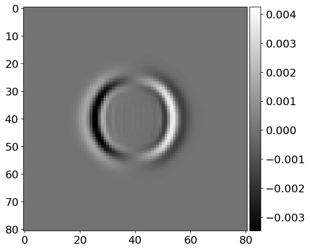
# NBVAL_SKIP
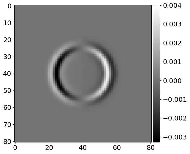
# Let's see what we got....
plot_image(v[0].data[0])
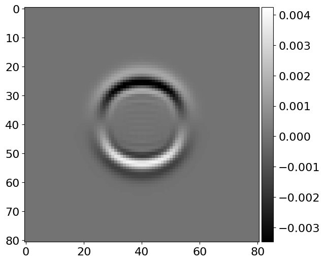
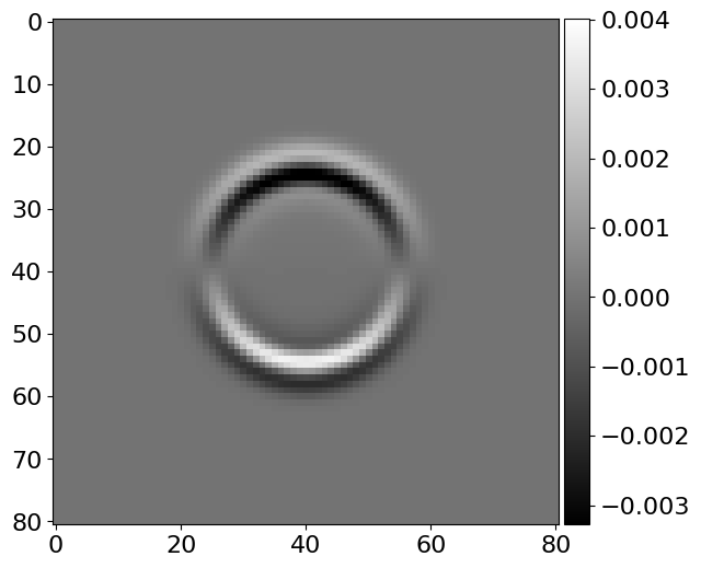
plot_image(v[1].data[0])
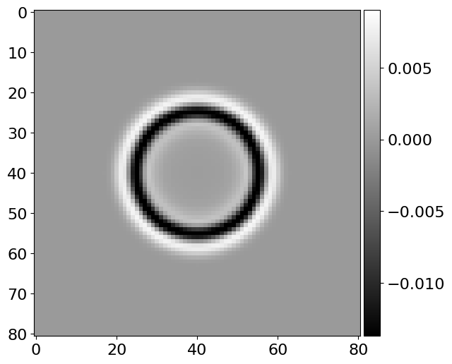
plot_image(p.data[0])
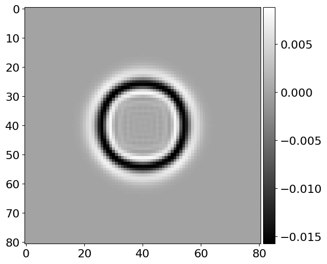
norm_p = norm(p)
assert np.isclose(norm_p, .35098, atol=1e-4, rtol=0)
# # 4th order acoustic according to fdelmoc
p4 = TimeFunction(name='p', grid=grid, staggered=NODE, space_order=4, time_order=1)
v4 = VectorTimeFunction(name='v', grid=grid, space_order=4, time_order=1)
src_p = src.inject(field=p4.forward, expr=src)
u_v_4 = Eq(v4.forward, solve(v4.dt - ro * grad(p4), v4.forward))
u_p_4 = Eq(p4.forward, solve(p4.dt - l2m * div(v4.forward), p4.forward))
# NBVAL_IGNORE_OUTPUT
op_4 = Operator([u_v_4, u_p_4] + src_p)
# Propagate the source
op_4(time=src.time_range.num-1, dt=dt)
Operator `Kernel` ran in 0.01 s


PerformanceSummary([(PerfKey(name='section0', rank=None),
  PerfEntry(time=0.0045040000000000045, gflopss=0.0, gpointss=0.0, oi=0.0, ops=0, itershapes=[])),
 (PerfKey(name='section1', rank=None),
  PerfEntry(time=0.0006889999999999998, gflopss=0.0, gpointss=0.0, oi=0.0, ops=0, itershapes=[]))])
# NBVAL_SKIP

# Let's see what we got....
plot_image(v4[0].data[-1])
plot_image(v4[1].data[-1])
plot_image(p4.data[-1])
norm_p = norm(p4)
assert np.isclose(norm_p, .33736, atol=1e-4, rtol=0)